Ion Conductivity

In situ measurements of nighttime polar (negative and positive) ion conductivity were performed by Holzworth et al. (1985). The polar conductivity values were found to be nearly equal ( $\sigma_{+}\!\simeq\!\sigma_{-}$) at most altitudes. Holzworth et al. (1985) measured ion conductivities which were well fit by an exponential scale height of 8.0 km below 40 km altitude and 11.1 km between 40 and 56 km altitude. The total ion conductivity ( $\sigma_{i}\!=\!\sigma_{+}\!+\!\sigma_{-}$) at 40 km was measured to be .

Holzworth et al. (1985) found a significant departure from the 11.1 km scale height above $\simeq$56 km altitude with a significant drop in $\sigma_{+}$ measured at 65 km altitude. The $\sigma_{i}$ profile above 56 km will be approximated by an exponential with the scale height determined from the measured $\sigma_{i}$ values at or near the endpoints of 56 km and 72 km. The total ion conductivity at 56 km using Equation 2.16 is 1.69$\times$10$^{-10}$ S/m while that at 70 km was measured by Holzworth et al. (1985) to be $\simeq$4.0$\times$10$^{-10}$ S/m. The exponential scale height based on these points would be about 16.3 km. The total ion conductivity profile is summarized in the equations below.

$$\sigma_{i} = 4.0\times10^{-11}e^{(\frac{z-40}{8.0})} \qua... ...riptstyle \frac{S}{m}}] \qquad \qquad z < \mbox{40~km} \quad$$ (2.15)

$$\sigma_{i} = 4.0\times10^{-11}e^{(\frac{z-40}{11.1})} \qu... ...riptstyle \frac{S}{m}}] \qquad \quad 40 \leq z < \mbox{56~km}$$ (2.16)

$$\sigma_{i} = 4.0\times10^{-10}e^{(\frac{z-70}{16.3})} \qua... ...riptstyle \frac{S}{m}}] \qquad \quad 56 \leq z < \mbox{72~km}$$ (2.17)

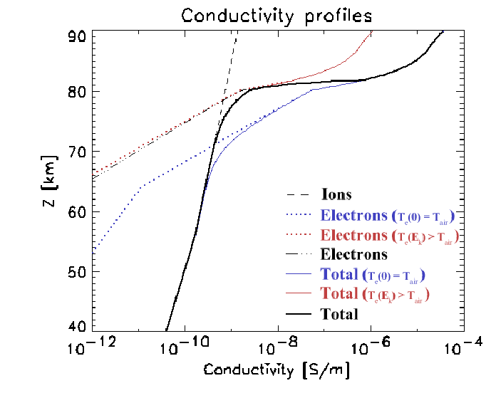
The dashed line in Figure 2.5 shows the ionic conductivity, $\sigma_{i}$, for 40-90 km altitude, based on Equations 2.15-2.17. Equation 2.17 was extended to altitudes above 72 km, even though Holzworth et al. (1985) did not obtain any measurements in that region. This extrapolation may be somewhat in error for altitudes of $\simeq$72-78 km. However, the increasing importance of the electron conductivity with increasing altitude will diminish the potential impact of such errors (see next section).

Figure 2.5: The ionic (dash), various electronic (dot and dash-dot), and corresponding total conductivities (solid) are shown in the graph above. An electron conductivity corresponding to: essentially ``cold'' electrons ( $T_e\!\simeq\!T_{air}$) is drawn in blue, ``hot'' electrons immersed in a breakdown field of $E_k$ ( $T_e\!\gg\!T_{air}$) is drawn in red, and a realistic electron $T_e$ based on a dipole field from the parent discharge, a near-breakdown field just below 80 km altitude, and a pre-existing relaxation time, is drawn in black (dash-dot). The corresponding total conductivities obtained by adding these electron conductivities with the ion conductivity is drawn with the same colors.