Uniformly Charged Disk

Sprites are primarily caused by +CGs which occur in the trailing stratiform region of mesoscale convective systems (MCSs) (Lyons, 1996; Boccippio et al., 1995). The sprite-producing +CGs may discharge horizontally-extensive positive charge regions which are known to exist near the $0^{\circ}$C isotherm within stratiform regions (Marshall and Rust, 1993; Marshall et al., 1996).

In order to assess the possibility of conventional breakdown onset as a function of parent discharge charge height and horizontal extent parameters, a static field approximation identical to that of Krehbiel et al. (1996) is implemented. In this approximation, the parent discharge is modeled as a uniformly charged disk of total charge $Q_{d}$, radius $R_{d}$, and altitude of $Z_{d}$ parallel to the ground. The electric field along the central axis above the disk can be readily determined, as shown below.

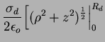
The solution to Poisson's equation ( $\nabla^{2}V\!=\!-\rho/\epsilon_o$) for a surface charge distribution is given by the formula:

$$V = \frac{1}{4\pi\epsilon_o}\int\frac{\sigma}{r}\,da$$

where $r$ is the distance along a vector to the infinitesimal area, $da$, of local charge density $\sigma$.

Using cylindrical coordinates for the disk; $da\!=\!{\rho}\,d{\rho}\,d{\phi}$, where $\rho$ is a radial distance from the disk center and $\phi$ is an angle around the disk. Assuming that $V$ is measured along the central axis; $r\!=\!(\rho^2+z^2)^{\frac{1}{2}}$, where $z$ is the height above the disk. Since the disk is assumed to be uniformly charged, $\sigma\!\equiv\!\sigma_d\!=\mbox{constant}$. 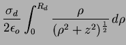Substituting,

$$V_d(z) = \frac{\sigma_d}{4\pi\epsilon_o}\int^{R_d}_0 \Bigg(\int^{2\pi}_{0}\frac{\rho}{(\rho^2+z^2) ^{\frac{1}{2}}} \,d\phi\Bigg)d\rho$$

$$= \frac{\sigma_d}{2\epsilon_o}\int^{R_d}_0 \frac{\rho}{(\rho^2+z^2)^{\frac{1}{2}}} \,d\rho$$

$$= \frac{\sigma_d}{2\epsilon_o}\Big[(\rho^2+z^2) ^{\frac{1}{2}}\Big\vert^{R_d}_0$$

$$= \frac{\sigma_d}{2\epsilon_o}\Big[({R_d}^{2}+z^2) ^{\frac{1}{2}}-z\Big]\;.$$ (2.21)

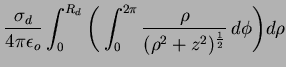
The electric field along the axis above the disk can be calculated from Equation 2.21 by using the electrostatic relationship $\vec{E}\!=\!-\nabla{V}$:

$$\vec{E_d}(z) = -\frac{\mbox{d}V_d}{\mbox{d}z}\;\hat{z}$$

$$= \frac{\sigma_d}{2\epsilon_o} \Bigg[1-\frac{z}{({R_d}^{2}+z^2)^{\frac{1}{2}}}\Bigg]\;\hat{z}$$ (2.22)

where $\sigma_d$ is the surface charge density on the disk,

$$\sigma_d = \frac{Q_d}{\pi{R_d^2}}\;,$$ (2.23)

which is assumed to be uniform.

Equations 2.22 and 2.23 provide a solution for $E_d(z)$ in terms of only $Q_d$, $R_d$, and the distance $z$ along the central axis from the disk. As was shown in Section 2.5.1, the actual electric field $E(Z)$ at some height $Z$ above the ground will be due to the source charge configuration and its multiple images. In this dissertation, the highest order disk-image pair used in the calculations corresponds to $i\!=\!2$ in Figure 2.7a. Thus, the expression for the electric field as a function of height along the central axis will be:

$$\vec{E}(Z) \cong \Big[ E_d(Z\!-\!Z_d)\;-\; E_d(Z\!+\!Z_d)\;+$$

$$\;\; E_d(2Z_{ledge}\!-\!Z\!-\!Z_d)\;-\; E_d(2Z_{ledge}\!-\!Z\!+\!Z_d)\;+$$

$$\;\;E_d(Z_{ledge}\!+\!Z\!-\!Z_d)\;-\; E_d(Z_{ledge}\!+\!Z\!+\!Z_d)\Big]\;\hat{k} \qquad \quad Z_d\!<\!Z\!<\!Z_{ledge} \qquad$$ (2.24)

where $Z_{ledge}$ is the altitude of the ionosphere conductivity ``ledge''. Equation 2.24 is valid only when the altitude of interest, $Z$, is greater than the altitude of the disk, $Z_d$.

It is well known in electrostatics that a dipole's field is proportional to the moment, $p\!=\!qd$, where $q$ is the charge magnitude and $d$ is the separation distance between the charges. The convention which is commonly used in sprite literature is to define the ``charge moment'' as the product of the total net charge with its mean height above ground, which would be one half the distance $d$ between the charge and its image. This convention will also be adopted in this study. Thus, the charge moment of the disk will be $Q_{d}Z_d$.

Figure 2.8 illustrates how the horizontal dimensions of the source charge region would affect the value of the electric field just below the base of the ionosphere ( $Z_{ledge}\!=\!81$ km) at $Z\!=\!78$ km. The charge moment, $Q_{d}Z_d$, was fixed for all of the plots. Thus, as $R_d$ is increased, $\sigma_d$ is decreased according to Equation 2.23) in order to keep $Q_d$ constant for a given $Z_d$. In reality, however, $\sigma_d$ may be somewhat fixed and thus more horizontally extensive discharges would produce a larger charge moment change, as was modeled by Marshall et al. (1996). The main purpose in this section is to determine how accurately the electric field below the base of the ionosphere can be determined based on charge moment measurements in which the discharge dimensions are not known. The charge moment will be kept fixed while the discharge dimensions are varied to see what effect this has on the electric field at high altitude.

Figure: The variation of the electric field at $Z\!=\!78$ km is shown as a function of disk radius, $R_d$, for a given charge moment, $Q_{d}Z_d$. The maximum electric field, $E_{max}$, corresponds to an extreme (and improbable) case of a point charge ($R_d\!=\!0$) at $Z_d\!=\!15$ km, the largest physically possible height (near the top of a convective turret). Larger $R_d$ and lower $Z_d$ will produce a smaller electric field ( $E/E_{max}\,<\,1$). However, decreasing $Z_d$ has only a minor effect, especially for realistic $Z_d$ of $5$ and $10$ km for which the electric field ratio differ by $\lesssim3\%$ at each $R_d$.

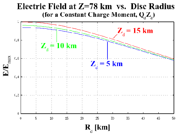For a given charge moment, Figure 2.8 shows that a more horizontally extensive flash will be less effective at initiating conventional breakdown. However, if the horizontal dimensions are sufficiently small ($R_d\!<\!20$ km), the decrease in electric field relative to the point charge approximation will be relatively minor ($<\!10\%$). In Chapter 3, it is shown that sprite-producing discharges may often meet this criterion.

Three different disk altitudes, $Z_d$, which roughly correspond to the range of physically possible values are plotted in Figure 2.8. The $5$ km altitude is close to that of the positive charge layer at or near the $0^{\circ}$C isotherm, typically between $4\!-\!5$ km altitude, within an MCS stratiform region (Marshall and Rust, 1993). An altitude of $10$ km is plotted since it has been used in the sprite-producing discharges modeled by Pasko et al. (1997b) and also represents a possible height of positive charge in a thunderstorm anvil (Marshall et al., 1989). An altitude of $15$ km would correspond to the upper part of a thunderstorm turret and is plotted merely for the purpose of comparison.

For a given charge moment, Figure 2.8 shows that the electric field is only weakly dependent on mean charge altitude for realistic altitudes. The difference between the $5$ and $10$ km plots is less than $3\%$ for all radii. This demonstrates the usefulness of the charge moment in assessing the likelihood of sprite initiation. One does not need to separate out the charge or height components. This will be fundamentally important for ELF measurements of sprite initiation thresholds (Chapters 4 and 5).