Infinite images

It is well known from electrostatic theory that a point charge placed above a conducting plane will cause charge to be redistributed on the plane's surface such that the potential will be constant there. Taking the potential to be zero on the surface, a charge of equal magnitude but of opposite sign to the source point charge can conceptually be placed an equal distance below the planar surface. The source charge and its image can be used to calculate the potential and hence the electric field vector anywhere above the conducting plane.

The situation becomes more complex when charge is placed between two parallel conducting planes. The charge will redistribute on the planes such that, conceptually, an image charge is formed behind each plane in the manner described previously. However, each plane will also respond to the redistribution of charge on the other plane and this will lead to the formation of ``images of images'' which are further displaced behind the respective conducting planes. The total number of images will be infinite, but the calculated electric field will be finite since each successive image charge is further away and the electric field contribution will decrease rapidly with distance.

A cloud-to-ground (CG) discharge will introduce a net charge at some average altitude $Z$. Figure 2.7a shows the index notation which is used in this work for the charge images. Assuming that a compact (``point'') region of negative charge were placed at an altitude of $Z\!=\!7.5$ km, surface charge rearrangement on the ground will lead to a positive image charge at $Z\!=\!-7.5$ km. It will be shown in Chapter 3 that $7.5$ km is a reasonable approximation for the altitude of charge removal in sprite-producing discharges. The source charge and its immediate image correspond to $i\!=\!0$ in Figure 2.7a.

Figure: a) A schematic diagram of the infinite images formed by a negative point charge placed above the Earth's surface. The indices at left correspond to increasing image pairs (approximately dipoles) of positive and negative charges. b) The rate of convergence at $Z\!=\!78$ km of the calculated electric field to a ``final'' electric field value is shown as a function of the number of successive image pairs included in the calculation (with $i\!=\!0$ corresponding to a calculation based only on the source and its below-ground image). The ``final'' electric field was calculated for a summation up to $i\!=\!100$.

Charge will rearrange on the nighttime ionosphere conductivity ledge at $Z\!\simeq\!81$ km (see Section 2.4.4) in response to the source charge and its image. The result is the $i\!=\!1$ image pair consisting of a positive image charge at $Z\!=\!81+(81-7.5)\!=\!154.5$ km and a negative image charge at $Z\!=\!81+(81+7.5)\!=\!169.5$ km. This, in turn, will lead to the $i\!=\!2$ pair of negative and positive image charges at $Z\!=\!-154.5$ km and $Z\!=\!-169.5$ km, respectively, and so on. The effect of the ionosphere is to enhance the electric field above the source charge. However, the electric field at ground-level is decreased by the presence of the ionosphere, as will be shown in Appendix C. This latter effect will be important for calculations based on electric field measurements presented in Chapter 3.

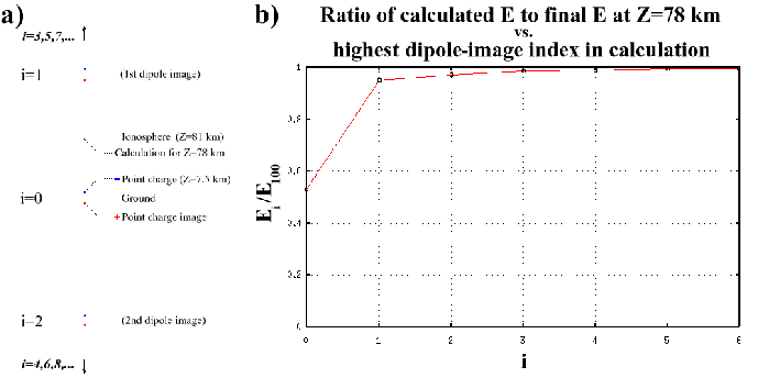
It will be shown in Section 5.2.4 that sprites often appear to initiate at 77-78 km MSL altitude. Figure 2.7b shows how the calculated electric field at $Z\!=\!78$ km varies with increasing image number in Figure 2.7a. The vertical axis is normalized such that a value of unity corresponds to the ``final'' electric field value, which was calculated for a summation up to the $i\!=\!100$ image pair. By $i\!=\!5$, the calculated electric field is within $1\%$ of the ``final'' electric field value. The rate of convergence of $E_i$ to $E_{100}$ is sufficiently fast that a much larger ``final'' $i$ value would not noticeably change the Figure 2.7b plot.

In this study, the theoretical electric field calculations for sprite altitudes implement a summation up to $i\!=\!2$. The electric field calculated in this manner will only be $\simeq3\%$ less than that based on an infinite summation.

It should be noted that the appearance of each successive image pair will be delayed by the amount of time that it takes the electric field (propagating at the speed of light) to traverse the Earth-ionosphere distance, ${\Delta}t\!\simeq\!81/300\!=\!0.27$ ms. As was shown by Pasko et al. (1999), the delayed appearance of the source charge's image below ground might significantly enhance electric fields aloft. For instance, if a charge were suddenly introduced at $Z\!=\!7.5$ km, an observer far above the charge would at first only experience the effects of this monopole, for which the electric field falls only as $r^{-2}$, before a less intense dipole-like dependency of about $r^{-3}$ appears due to the image. The time delay between the monopolar and dipolar field dependency would be twice the height of the charge divided by the speed of light (since the electric field must propagate down and then back up to the observer). For a charge at $Z\!=\!7.5$ km: ${\Delta}t\!=\!0.05$ ms. This time difference is not much less than the duration of the return stroke, which is typically $\sim$75-230 $\mu$s (Uman, 1987, pg. 124). This retardation effect could significantly lower the sprite initiation threshold (Pasko et al., 1999) from the quasi-electrostatic predictions of the following sections.