Effect of Ionosphere on Static Field Measurements

It was shown in Section 2.5.1 that charge images due to the presence of the ionosphere increased the electric field above the source charge. It was also shown that the total number of images in a static electric field calculation was infinite, though the electric field rapidly converged with increasing image index to a final value at altitudes where sprites were likely to initiate. In this section, the effect of ionospheric images on static electric field observations near the ground at some distance from the source will be examined. The image index notation will be the same as in Figure 2.7a.

The distance to the estimated charge removal center of the sprite-producing discharges listed in Table 3.1 was about 80 km. Figure C.1 shows the convergence of the calculated electric field at 80 km range to a ``final'' electric field value as a function of the image index. Unlike the electric field at high altitude (see Figure 2.7b), the electric field at ground level is decreased by the presence of the ionosphere.

Figure: The electric field is calculated at ground-level ($Z\!=\!0$ km) at a range, $r$, of $80$ km from the source charge. The rate of convergence of the calculated electric field to a ``final'' electric field value is shown as a function of the number of successive image pairs included in the calculation (with $i\!=\!0$ corresponding to a calculation based only on the source and its below-ground image). The ``final'' electric field was calculated for a summation up to $i\!=\!100$.

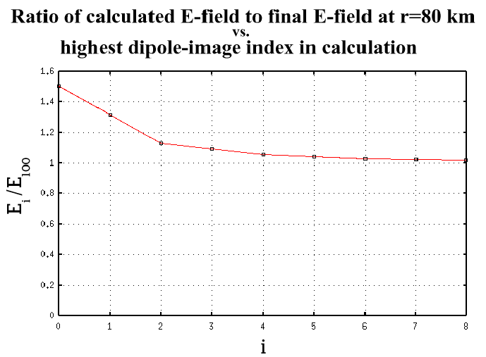The calculated electric field converges to a final electric field value in Figure C.1, but the rate of convergence at a range of 80 km at ground level is slower than the rate of convergence at an altitude of 78 km MSL above the discharge (see Figure 2.7b). However, one should not use a large summation when attempting to determine a charge moment from an observed electric field since the images are not set up instantaneously. Rather, each successive image is delayed by at least the light propagation time between the ground and the ionosphere ( ${\Delta}t\,\simeq\,81/300\,=\,0.27$ ms).

In order to calculate the charge moments in Table 3.1 at delays of 1 and 4 ms after the return stroke, the product of the number of images with the light propagation time between the ground and ionosphere was not allowed to be greater than the post return stroke delays. To complicate matters, the charge moment of the sprite-producing discharges increased throughout the interval after the return stroke instead of being ``suddenly'' introduced at $t=0$. Thus, the number of images used in the static field calculation had to reflect the fact that some of the quasistatic electric field change might have occurred with less time for images to form relative to earlier portions of the field change. For the 1 ms delays, the highest image index included in the charge moment calculation shown in Table 3.1 was 3. The highest image index for the 4 ms delays was 7.

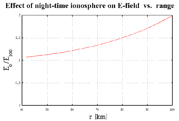
Near the source charge the effect of the ionosphere can be neglected since the electric field from the charge will dominate. As the range to the source is increased, the effect of the ionosphere images will become increasingly important. The ratio of the electric field calculated without the presence of an ionosphere, $E_0$, to the ``final'' electric field, $E_{100}$, is shown as a function of range in Figure C.2. At 40 km range, the ionosphere only decreases the static electric field by at most 7%. At 100 km range, however, the ionosphere reduces the static electric field by about a factor of two.

Figure C.2: The ratio of the electric field without the presence of the ionosphere to the field calculated with an ionosphere at $Z=81$ km (night-time) is shown as a function of range.