Langmuir Laboratory, 1997

Electric and magnetic field data was acquired on the Magdalena Ridge at Langmuir Laboratory in 1997. The electric field would have been significantly enhanced on the ridge. The NLDN data will be used to determine the amount of electric field enhancement caused by the ridge and to properly calibrate the magnetic field instrument.

The magnetic field instrument was borrowed from Chris Barrington-Leigh of Stanford University. The magnetic field sensor consisted of a wire which was looped multiple times around the perphery of a square frame. The absolute sensitivity of the wire-loop and amplifier was calibrated. It was found that a change of 1.5 nT in the magnetic field component normal to the plane of the wire loop produced an output of $\sim\,$1 V. However, significant errors may exist in the calibration procedure which was used in 1997 (C. Barrington-Leigh, private communication, 1998).

A well known result from electrodynamics is that at sufficient distances from an electromagnetic source, the magnetic field is related to the electric field by the simple relationship, $B=E/c$. Substituting this relationship into Equation B.3 gives:

$$B_p = \frac{\mu_o\,I_p\,V_{rs}}{2\,\pi\,r\,c}\$$ (B.7)

where $B_p$ is the peak magnetic field and $\mu_o$ is the free-space permeability ( $\mu_o\epsilon_o=1/c^2$).

Near the ground, the electric field will be vertical while the magnetic field will be tangential to a circle centered on the current source. The magnetic field which is measured by the instrument is the component which is normal to the plane of the loop. $B_p$ is related to the measured peak magnetic field, $B_{pm}$, by the trigonometric relationship:

$$B_{p} = \frac{B_{pm}}{\sin{({\theta}_l - {\theta}_s)}}$$ (B.8)

where $\theta_l$ is the azimuth of the normal to the plane of the loop and $\theta_s$ is the azimuth to the source current. The null in sensitivity ( $B_{pm}\rightarrow0$) occurs when these azimuths are either identical or $180^\circ$ apart.

The $\theta_l$ value could have been determined from a compass, but this was not done accurately. The loop orientation can be found accurately by determining where $\theta_l$ produces measured $B_p$ values which are consistent with the predicted $B_p$ values.

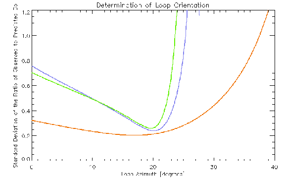
Figure B.6 shows the standard deviation of the ratio of $B_p$ calculated from Equation B.8 based on measured $B_{pm}$ values and the $\theta_s$ values provided by NLDN to $B_p$ calculated from Equation B.7 based on the NLDN $I_p$ and $r$ values. The standard deviation of the ratio is shown as a function of $\theta_l$ for the three different days on which high-speed video of sprites was obtained: October 3 (blue), October 6 (red), and October 7 (green) 1997. The agreement between the magnetic field values calculated by the two techniques increases as the standard deviation decreases. The minimum standard deviation of the ratio near $\theta_l=20^{\circ}$ azimuth corresponds to the orientation of the normal to the plane of the loop on all three days. The October 3 and 7 data is particularly sensitive to loop orientation since there were storms near one of the two nulls in loop sensitivity on both days, albeit for a different null on each day.

Figure B.6: The standard deviation of the ratio of the peak magnetic field, $B_p$, calculated from measurements to $B_p$ calculated from NLDN data for three different days: October 3 (blue), October 6 (red), and October 7 (green) 1997. The minimum near $20^\circ$ azimuth corresponds to the orientation of the normal to the plane of the loop on all three days.

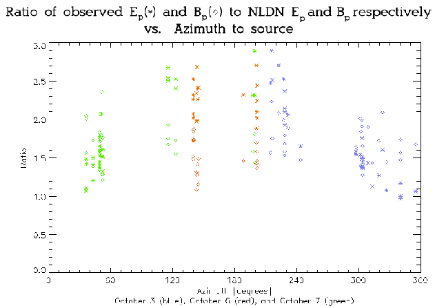
Equations B.7 and B.8 were used to calculate the expected $B_p$ values based on NLDN data and a loop orientation of $20^{\circ}$. Equation B.3 was used to calculate the expected $E_p$ values based on NLDN data. Figure B.7 shows the ratio of the observed $E_p$ and $B_p$ values to the $E_p$ and $B_p$ values calculated from NLDN data, respectively, as a function of azimuth to the stroke. The observed $B_p$ values are about 1.6 times greater than predicted and this enhancement factor appears to be independent of the azimuth to the source.

Figure B.7: The ratio of the observed $E_p$ and $B_p$ values to the $E_p$ and $B_p$ values calculated from NLDN data respectively, is shown as a function of source azimuth. The observed $B_p$ values are about 1.6 times greater than predicted from NLDN data for all source azimuths. The observed $E_p$ values are also enhanced over the values predicted from NLDN data, but the enhancement factor is a function of source azimuth.

A new calibration factor of $1.5/1.6=0.94$ nT/V was used to convert digitized magnetic data (with a known conversion factor between digital units and volts) to corresponding magnetic field values. The charge moment change calculations reported in Chapter 5 were based on the $0.94$ nT/V conversion factor. The net effect of the NLDN-based calibration was to reduce the calculated charge moment values by about 40% from those based on the calibration of the magnetic field instrument.

No attempt was made to account for attenuation (see Equation B.4) in the calculations, since the attenuation exponents for the region around Langmuir are not known. However, NLDN strokes between 50 and 200 km range were analyzed using the Florida-based attenuation factors to see how including attenuation might effect the calibration. It was found that the observed $B_p$ values were about 1.85 times greater than the predicted $B_p$ values, an enhancement which is only 16% greater than the enhancement which was calculated without any attenuation.

The observed $E_p$ values were roughly a factor of two greater than the $E_p$ values based on NLDN data. The electric field enhancement was expected since the electric field meter was on a mountain ridge. However, the variation of the enhancement factor with source azimuth was not expected. It is speculated that this variation may be due to the presence of nearby metallic trailers and other conductive obstructions. The magnetic loop antenna was placed in an open field further away from the balloon hangar, so it would not have been subject to the same complications.