Relaxation Time during the Day

The nighttime relaxation time profile was derived and shown in Section 2.4.4. In this section, we will estimate $\tau_{r}$ as a function of height around the time of the daytime sprites. The results will then be used in the next section to estimate the initiation altitude of the sprites.

Figure 4.6a shows the IRI-95 model (Rawer et al., 1978) of electron number density ($n_{e}$) relative to local ground-level sunset over South Texas on August 14, 1998. The base altitude of the model output is 65 km for daylight hours and 80 km for night. A significant change in $n_{e}$ occurs within $\pm$3 hours of sunset, with the greatest change being at sunset when the change in incident solar flux is greatest. The dashed line in Figure 4.6a is the IRI-95 $n_{e}$ profile at 23:19:48 UT, the time of the first sprite event. The solid line in Figure 4.6b shows $\tau_{r}$ based on the IRI-95 $n_{e}$ profile and a ``cold electron'' assumption (see Pasko et al. (1997b)) for 65-70 km altitude at 23:19:48 UT. Note that although $n_{e}$ at the time of the sprites was significantly less than at midday, the corresponding $\tau_{r}$ was still very small.

Figure 4.6: a) The IRI-95 model of electron density ($n_{e}$) as a function of time in hours relative to sunset over S. Texas on August 14, 1998. The dashed line shows the IRI-95 $n_{e}$ at the time of the first sprite. b) The relaxation time ($\tau_{r}$) at the time of the first sprite, with the IRI-95 model (thick solid line) extrapolated below 65 km (thick dashed line) and incorporating the effects of different ion concentrations of Holzworth et al. (1985) (Profile A) and Hale (1994) (Profile B) below 60 km. The vertical dotted lines show the range of daytime sprite delays ($t_{s}$).

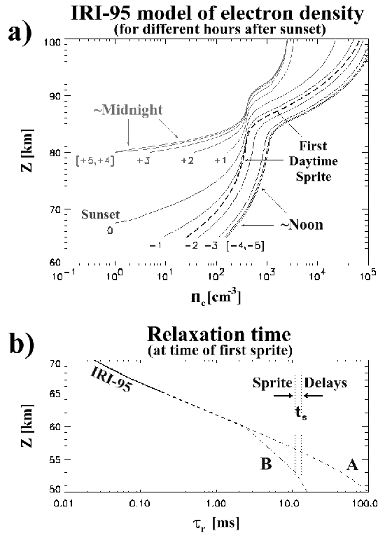The thick dashed line in Figure 4.6b shows the IRI-95 $\tau_{r}$ extrapolated down to 60 km altitude using the $\tau_{r}$ scale height at 65 km altitude. Below 60 km, ion conductivity begins to dominate over the electron conductivity (Reid, 1986). The thin dashed line (profile A) in Figure 4.6b below 60 km is based upon combining the IRI-95 electron conductivity extrapolation with the experimentally measured ion conductivity of Holzworth et al. (1985). The dot-dash line (profile B) in Figure 4.6b is an interpolation between the IRI-95 $\tau_{r}$ profile and Hale's mid-latitude $\tau_{r}$ profile for 53 km altitude and below (Hale, 1994). The vertical dotted lines in Figure 4.6b denote the range of daytime sprite initiation time delays ($t_{s}$: 11.0-13.2 ms) reported in this study. Note that $\tau_{r}$ exceeds all $t_{s}$ below $\simeq$56 km altitude for Profile A but does so only below $\simeq$51 km altitude for Profile B.