1976 U.S. Standard Atmosphere

In 1953, the United States Committee on Extension to the Standard Atmosphere (COESA) was formed to assemble information on atmospheric parameters at altitudes traversed by suborbital rockets. One result of this effort was a mid-latitude (45 $^{\circ}$ N) mean atmospheric profile published in U.S. Standard Atmosphere, 1962. COESA provided information, graphs, and tables of the latitudinal, seasonal, and diurnal variations of atmospheric parameters in U.S. Standard Atmosphere Supplements, 1966. The 1962 U.S. Standard Atmosphere model was updated when the United States National Oceanic sand Atmospheric Administration (NOAA) released U.S. Standard Atmosphere: 1976. The 1976 U.S. Standard Atmosphere is identical to the 1962 U.S. Standard Atmosphere for altitudes below 50 km, but differs for higher altitudes.

Fortran code for the 1976 U.S. Standard Atmosphere was obtained off of the web (http://gate.cruzio.com/ $\,\tilde{ }$ pdas/atmosf90.htm). The code was converted to Octave and IDL to interface with conventional breakdown (Section 2.5) and refraction (Appendix B.5) calculations respectively.

A critical atmospheric parameter for conventional breakdown models is the air number density,

, since the breakdown field,

, scales directly with

(see Sections 2.2.2 and 2.2.3). The scale factor relative to sea level will be the ratio of

to that at sea level,

. Figure 2.3a shows the 1976 U.S. Standard Atmosphere model of air density ratio as a function of height. The air density decreases exponentially with height.

**Figure 2.3:** a) The ratio of the density of air to that at sea level is plotted as a function of height. b) The temperature is plotted as a function of height. The different atmospheric regions correspond to regions of increasing/decreasing temperature with respect to height.
$\begin{figure}\begin{center} \par\epsfig{file=eps/1976_atmos.eps,width=6in}\par\par\par\end{center}\end{figure}$

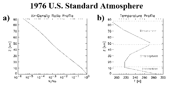The 1976 U.S. Standard Atmosphere model of temperature as a function of altitude is shown in Figure 2.3b. The approximate altitude range of the troposphere, stratosphere, and mesosphere are shown on the plot. Each successive layer alternates between polarities for the vertical temperature gradient. Above $\simeq$ 86 km altitude, the temperature slope becomes positive again (not shown), which corresponds with the approximate base of the thermosphere. The changes in temperature with respect to height produce small ``wiggles'' in the air-density ratio in Figure 2.3a, which otherwise would be a straight line.