01:42:57 UT Sprite-producer

The first sprite cluster was observed at 01:42:57 UT, about a half-hour after video observations began. The development of the sprite cluster is shown in Figure 3.3. The light integration period for the first image began at 160$\pm$4 ms and ended $1000/60\!=\!16.7$ ms later at 177$\pm$4 ms after 01:42:57 UT.

A single sprite appeared in the first video field in Figure 3.3, one field before the remaining 3 sprites. The first sprite bloomed in the next field. This indicates that it was still in the process of developing at the end of the first video field. A 50.2 kA +CG had occurred at 171.7 ms and 71.1 km range. From the video frame timing, the sprites visible in the second field developed no sooner than 1 ms after the +CG and no later than 9 ms afterwards. As Table 3.1 shows, the cumulative charge moment change increased significantly from 1 to 4 ms after the return-stroke onset. Unfortunately, there were $\pm$4 ms timing errors due to the image saturation by the LED which made it difficult to pinpoint the time of an LED transition (see Appendix B.4.2 for an example of how video timing is determined from LED transitions). These timing errors made it impossible to determine a possible sprite initiation threshold with greater accuracy than derived earlier in Section 3.5.

All of the sprites reached maximum brightness in the second video field. The sprites faded into the third video field and continued to fade until they were barely visible in the fifth field. The total optical duration of the sprite event was $\sim$70 ms.

The 3-dimensional development of the 01:42:57 UT sprite-producing flash relative to NEXRAD radar reflectivity contours is shown in the lower half of Figure 3.3. The NEXRAD radar was based in Melbourne, Florida, to the southeast of the MCS. The displayed elevation scan corresponded to an altitude of $\sim$5 km on the southeast side of the storm, and increased to $\sim$8 km on the northwest side. The contours are incremented at 10 dBZ intervals starting at 0 dBZ.

Figure 3.3: The temporal development at 17 ms intervals of the 01:42:57 UT sprite cluster is shown at top as seen through a wide angle lens. The LDAR data is plotted on top of NEXRAD reflectivity at bottom and is rainbow-colored from blue to red with respect to time. The reflectivity is contoured at 10 dBZ intervals starting with 0 dBZ. Note that the flash is mostly confined within 20+ dBZ reflectivity, but does not traverse the entire 20+ dBZ region.

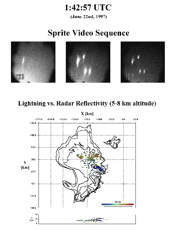The higher reflectivity regions occurred along a southwest-northeast line on the southern edge of the MCS are the convective cores. The stratiform region trails behind the northern edge of the line while new cells formed on the southern edge, as shown in Figure 3.2. This asymmetric development pattern is identical to that of asymmetric Oklahoma MCSs which are known to be more likely to produce tornadoes and hail than their symmetric counterparts (Houze et al., 1990).

It is known from laboratory experiments that electrical discharge propagation is spatially correlated with the locations of space charge regions (Williams et al., 1985). Thus, lightning channels mapped by the KSC LDAR should give an indication of charge location.

The flash began in a high reflectivity region of $\sim$40 dBZ (at $\sim$5 km altitude) within a convective cell on the eastern edge of the MCS. It then propagated into the lower reflectivity stratiform region. The flash was mostly confined within the $\gtrsim$20 dBZ reflectivity region, but did not traverse the entire $\gtrsim$20 dBZ region. The flash development relative to radar reflectivity was very similar to that documented by the KSC LDAR for smaller Florida storms (Stanley et al., 1996a; Maier et al., 1995b).

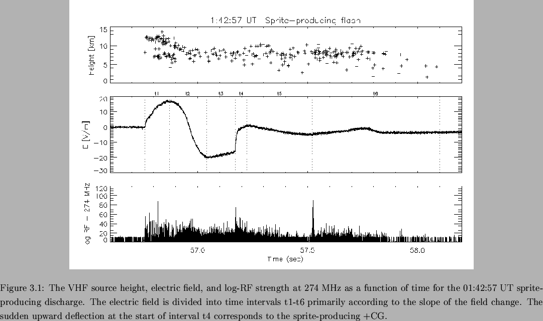
The temporal and spatial development characteristics of the sprite-producing flash are shown in Figures 3.4 and 3.5. The duration of the flash was about 1.3 s. The electric field was measured at the interferometer site by a slow antenna with a long relaxation time of $\sim$10 s. The log-RF at 274 MHz is shown in 8-bit digital units in Figure 3.4. The noise level of the log-RF is at $\sim$10 units. The dropouts in log-RF data are due to the RF-thresholded data acquisition mode which was in effect for this flash.

The initial upward deflection of the electric field was caused by the upward (and possibly towards the observer) transport of negative charge during the initial portion of the intracloud discharge. This transport of negative charge by negative leaders propagating into the upper positive charge region of the convective cell makes negative charge more ``visible'' to distant ground observers, thus increasing the vertical electric field at a distance. This initial portion of the flash is designated as interval ``t1''.

The subsequent downward deflection of the electric field in interval t2 of Figure 3.4 was due to the transport of negative charge out into the positively charged anvil in a direction away from the slow antenna. The outward motion is clearly evident in Figure 3.5b by the temporal development of inferred negative leaders away from the interferometer and observation site at $[x,y]\!=\![0,0]$, as indicated by the rainbow-color progression from blue (sooner) to red (later). The flash developed over a $\simeq$40 km distance in the 170 ms interval of t2. This corresponds to an average negative leader velocity of 2.4$\times$10$^5$ m/s, which is consistent with negative leader velocities in ordinary ICs (Shao and Krehbiel, 1996), spider-lightning discharges, (Mazur et al., 1998), and -CGs (Uman, 1987, pg. 83).

The negative breakdown developed into a region of 20-30 dBZ reflectivity within the stratiform region, as indicated by Figure 3.3. The decrease in altitude of the negative breakdown at the start of interval t2 in Figure 3.4 is in excellent agreement with the decrease in average positive charge altitude from $\simeq$11 km in an MCS convective core to $\simeq$8 km in the stratiform region (MacGorman and Rust, 1998, pg. 267). A horizontally extensive flash observed by the New Mexico Tech Lightning Mapping Array also developed in a similar fashion within an MCS in Oklahoma (Krehbiel et al., 2000).

A bilevel structure in the IC flash is clearly evident in Figure 3.4 for time intervals t1 and t2. The initial development and bilevel nature are consistent with previous VHF observations of IC flashes with the upper level corresponding to the positive charge region and the lower level to the negative charge region (Shao and Krehbiel, 1996). The lower level VHF sources may correspond to negative polarity recoil events which delineate the tracks of positive leaders (Mazur and Ruhnke, 1993). Support for this comes from VHF measurements which have failed to detect positive leaders from close triggered lightning, though negative polarity breakdown events propagating back along the inferred positive leader channel locations are readily detected (Krehbiel et al., 1994; Stanley et al., 1994; Shao et al., 1996).

Figure 3.5: The spatial development of the 01:42:57 UT sprite-producing discharge as a function of time. The VHF sources ($\Diamond$) are rainbow-colored from blue to red according to elapsed time within the respective time interval. VHF sources from previous intervals ($\cdot$) are purple. The +CG location (+), LDAR-indicated sprite-producing discharge center (*), and sprite locations (x) are shown within time interval t4. The maximum range error estimates for the sprite locations are indicated with lines. Note that many of the sprites appear to lie at the periphery of the parent discharge.

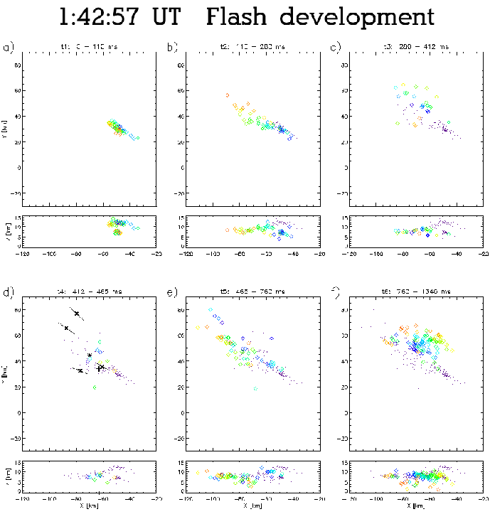The VHF activity in the lower level of the bilevel IC flash appeared to stop near the beginning of time interval t2. This may indicate that the positive leaders have stopped propagating. However, the relationship of VHF source occurrence to positive leader propagation is poorly understood at the present time. Thus, it is not clear when, or even if, the positive leaders have ceased, though the lack of VHF sources suggests that they have ceased. Figure 3.5c shows that only a single VHF source occurred in the lower level in time interval t3.

The recovery of the electric field in interval t3 is partly due to the ``right-turn'' and tangential-motion taken by the negative leaders in Figure 3.5c. This recovery is also the strongest evidence that older channel segments became resistive, consistent with the interpretation that the positive leaders had stopped propagating. If the entire channel structure was still conductive, the outward transport of negative charge through the closer channel structure would have continued to decrease the electric field at the observation site.

The horizontal extent of the flash did not grow much beyond interval t3, as an inspection of Figure 3.5d-f shows. This indicates that the negative leaders essentially stopped near the periphery of the 20 dBZ reflectivity region, as was discussed earlier. The sources at the end of the interval t3 occurred on the southern end of the horizontally expansive region near the +CG strike point. The significance of this is not understood.

The +CG occurred at the start of interval t4. There is no clear indication in the LDAR data that the positive leader to ground was detected, particularly since there were no data points below $\sim$6 km up to the time of the +CG. This is not unexpected, since previous measurements of +CG leaders at VHF by the interferometer show that they radiate only weakly (Mazur et al., 1998).

Initial triangulation studies of sprites indicated that the upper terminal height was 88$\pm$5 km (Sentman et al., 1995). Triangulation of numerous columniform sprites by Wescott et al. (1998) determined that their average upper terminal height was 87 km, but could range from 81-89 km. To determine the locations of these sprites, a terminal height of 87$\pm$6 km was used. The camera orientation was determined precisely based on stellar locations (see Appendix B.3.1). Thus, the location errors will primarily be range errors due to $\pm$6 km height errors. Since the elevation angle to the top of the sprites was on the order of 45$^{\circ}$, the range errors will be approximately the same as the terminal height errors.

The most probable locations of the sprites is shown in Figure 3.5d along with a range error estimate for the locations. Surprisingly, the plan position of two sprites appear to lie at the periphery of the discharge while the northernmost sprite appears to lie just beyond the apparent discharge boundary. The fourth sprite was almost directly over the +CG strike point. The first sprite which appeared in Figure 3.3 was located west of the +CG along the southern edge of the discharge.

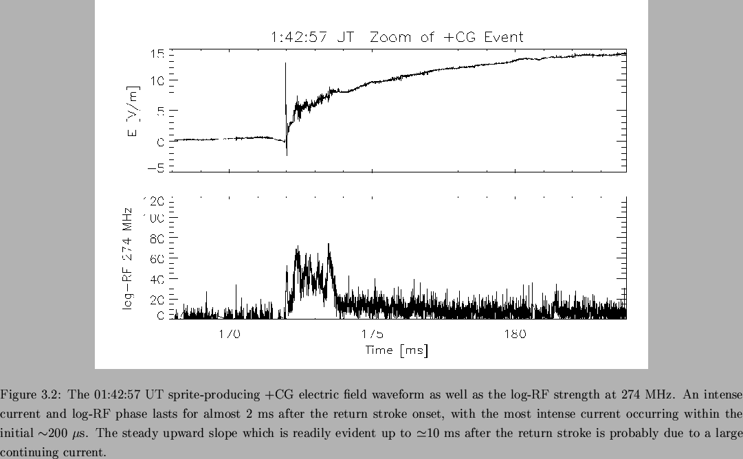
Figure 3.6 shows an expanded plot of the electric field and 274 MHz log-RF around the time of the +CG. The LDAR data is not shown since there were too few data points within the time interval. The electric field was obtained by de-drooping the fast antenna data (which has a higher sample rate than the slow antenna) so that the static field change component of the slow antenna was accurately reconstructed for the time intervals around the +CGs shown in this work. The 60 Hz AC and higher harmonics were (incompletely) subtracted from the final waveform.

A sudden increase in the electric field occurred about 200 $\mu$s after the return stroke according to Figure 3.6. The electric field increased with a substantial slope and noisy bursts superimposed until about 2 ms after the return stroke. This phase of the discharge was accompanied by strong VHF radiation. After 2 ms, the electric field continued to increase due to a persisting intense continuing current until $\sim$10 ms after the discharge, when the slope became more gradual. The more gradual slope may correspond to only horizontal movement of charge after the cessation of continuing current or could be due to a significantly weakened continuing current.

The log-RF activity is enhanced throughout the entire interval after the +CG. It is the negative leader activity which supplies the current during the continuing current phase of the discharge, so this is expected.

The LDAR-indicated charge center used in Table 3.1 was near the middle of the sprite cluster and is much closer to the cluster center than to the location of the +CG. The charge moment change based on this charge location was 265 C$\cdot$km at 1 ms. Figure 3.6 shows that most of this charge moment change occurred within the initial $\sim$200 $\mu$s, thus retardation effects will be important and the electric field will be briefly higher than expected from quasi-electrostatic theory (see Section 2.5.1). However, it is not clear how this could produce the observed pattern of sprite initiation, particularly since the field from a monopole has a weaker radial dependency than a dipole and seemingly would be even less likely to produce high fields near the periphery of the discharge.

Figure 3.5 shows the remaining development of the flash in intervals t5 and t6. The x-z plots indicate that many of the VHF sources were associated with channels which propagated down from $\simeq$8 km altitude to $\simeq$4 km altitude, or to about the height of the 0$^{\circ}$C isotherm. The lower altitude sources were likely associated with spider-lightning discharges, which can be observed to ``crawl'' below cloud base or just above cloud-base (Marshall et al., 1989). Such spider-lightning discharges typically propagate at about 4 km altitude, presumably through a stratified positive charge layer, and are composed of negative leaders (Mazur et al., 1998).

The measurements presented here indicate that the charge removed for this sprite-producing +CG was associated with positive charge higher up in the stratiform region, rather than near the 0$^{\circ}$C isotherm. The average height of the charge region according to Figure 3.7 was $\sim$7.5 km MSL. Based on the LDAR range-based charge moments (Table 3.1), the charge transferred to ground would have been 35 C at 1 ms and 64 C at 4 ms after the return stroke. The average current for these intervals would have been 35 kA and 16 kA respectively. Such high average currents are not unusual for +CGs, as indicated by current (Berger, 1972) and multi-station electric field (Brook et al., 1982; Krehbiel, 1981) measurements.

Figure 3.7: The density of VHF sources in 500 m height bins is shown above for the 01:42:57 UT flash. The VHF sources above 10 km altitude were associated with the initial IC development while those below 6 km occurred later in the flash, after the sprites. Factoring in a small systematic error which increases the heights by $<$1 km (Section 3.2.1), the average charge removal height of the sprite-producing +CG was between 7-8 km altitude.